Dictionaries

CS240E: Data Structures and Data Management (Enriched)

David Duan, 2019 Winter

Motivation

Dictionary ADT

A dictionary is a collection of key-value-pairs (KVP) with operations

search(k), or findElement(k)
insert(k, v), or insertItem(k,v)
delete(k), or removeElement(k)

$O(1)$ $O(1)$ time and all keys in a dictionary are distinct.

Naive Implementations

Unsorted $O(1)$ $O(n)$ $O(n)$ delete.
Sorted $O(n)$ $O(\log n)$ $O(n)$ delete.

Binary Search Trees

A BST is a binary tree (where each node stores a KVP) that satisfies the BST order property: key(T.left) < key(T) < key(T.right) for all node T.

Operations

Search

If the node is NIL, return.
If current node has a key equal to the target key, return current node.
If current node has a key less than the target key, search the left subtree.
Otherwise, search the right subtree.

Insert

If the node is NIL, construct a new node with given KVP.
If the node's key equals the target key, renew its value.
If the node's key is less than the target key, insert KVP to the left subtree.
Otherwise, insert KVP to the right subtree.

Delete

If the target node is a leaf, remove it.
If the target node only has one child, promote its child to its position.
Otherwise, swap the node with its in-order successor (or predecessor), which is the left-most node in its right subtree, then delete the node (which is now a leaf).

Remark

lazy-deletion $d$ $d > n$ $\Theta(n)$ $O(1)$ $n$ $O(n)$ time. Note that when a node is marked as "dummy", you might still want to preserve its key for comparisons.

Analysis

$h$ $h(\varnothing) = -1$ $h(x) = 0$ $x$ is a singleton.

$h = (n-1) \implies h \in \Theta(n)$ .
$h \approx \log n\implies h\in \Theta(\log n)$ .
$h \in \Theta(\log n)$ , see below.

Average Case Analysis

$\{0, \ldots, n-1\}$ $i$ .

$\{0, \ldots, i-1\}$ $\{i+1, \ldots, n-1\}$ $i-1$ $n - i - 1$ .

$c_n$ $n$ $c_n = 1 + \max\{c_i, c_{n-i-1}\}$ $i$ is unknown, we take the expected value of the expression above:

c_n = 1 + \sum_{i=0}^{n-1} \frac{1}{n} \max\{c_i,c_{n-i-1}\}.

$i$ $0$ $n-1$ .
$1/n$ $i$ $1/n$ $n$ possible values.
$\max\{c_i, c_{n-i-1}\}$ : we want to consider the maximum of two subtrees.

$T(n) = c_n$ $i$ $n/4$ $3n/4$ $1/2$ $3n/4$ $T(n)\leq 1 + T(3n/4)$ in this case:

\begin{align*} T(n) &\leq 1 + P(\text{$i$ in $[n/4, 3n/4]$}) \cdot T(3n/4) + P(\text{$i$ not in $[n/4, 3n/4]$}) \cdot T(n) \\ & \leq 1 + \frac{1}{2}T(3n/4) + \frac{1}{2}T(n) \\ \frac{1}{2}T(n) &\leq 1 + \frac{1}{2}T(3n/4) \\ T(n) &\leq O(1) + T(3n/4) \in O(\log n). \end{align*}

$\Theta(n)$ proof.

Lower Bound for Search

$\Omega(\log n)$ for comparison-based search using decision trees.

$n$ $n$ $n$ $\log n$ $\Omega(\log n)$ $\square$

Random BST

random binary search tree $n$ $x_0, \ldots, x_{n-1}$ $0, \ldots, n-1$ , and add its elements, one by one, into a BST.

$O(n \log n)$ $n$ $O(\log n)$ expected time.

Treaps

$O(\log n)$ .

The idea is to use randomizationexpected $O(\log n)$ .

Every node of a Treap maintains two values:

Key which follows standard BST ordering (left smaller and right greater)
Priority which is a randomly assigned value that follows max-heap ordering property.

In short, a Treap follows both BST ordering property and max-heap ordering property.

Operations

Search(k) $O(h)$ .

Insert(k)

$\{0, 1, \ldots, n-1\}$ $k$ .
$(k,p)$ as an ordinary BST.
Fix the priority (max-heap order property) with rotations, i.e., locally rearrange the BST while keeping the BST order property.

Rotation

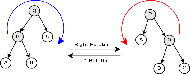
The tree rotation renders the inorder traversal of the tree invariant. For more details, check out rotation section on AVL tree.

Note that, because of rebalancing rotations, Treaps hide insertion orders.

Analysis

$\mathbb E(h) \in O(\log n)$ .

AVL Tree

height-balance $L$ $R$ $1$ $h(R)- h(L) \in \{-1, 0, 1\}$ $-1$ left-heavy $0$ balanced $+1$ right-heavy $n$ $\Theta(\log n)$ $\Theta(\log n)$ in the worst case.

Every node of a Treap maintains two values:

Key which follows standard BST ordering (left smaller and right greater).
Height $0$ ).

$h(R) - h(L)$ at each node, which may save some space but the code gets more complicated.

$\Theta(h)$ just as ordinary BSTs. We cover AVL-insertion extensively.

Insertion

Procedure

Insert as for a BST.
$\pm 2$ $z$ $z$ unbalanced.
$z$ $y$ $x$ $z, y, x$ $\{x,y,z\}$ to the root.

Pseudocode


x
1
AVL-insert(r, k, v)
2
r: root of the tree
3
(k, v): KVP to insert
4
5
1.  z <- BST-insert(r, k, v)
6
2.  z.height <- 0
7
3.  while (z is not the root)
8
4.    z <- parent of z
9
5.    if (|z.left.height - z.right.height| > 1) then
10
6.      let y be the taller child of z (break ties arbitrarily)
11
7.      let x be the taller child of y (break ties to prefer left-left or right-right)
12
8.      z <- restructure(x)  // see rotation
13
9.      break
14
11.   setHeightFromSubtrees(z)


xxxxxxxxxx
3
1
setHeightFromSubtrees(u)
2
1.  if u is not an empty subtree
3
2.    u.height <- 1 + max(u.left.height, u.right.height)

Rotation

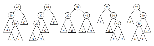
There are many different BSTs with the same keys. Our goal is to change the structure among these three nodes without breaking BST order property, so that the subtree becomes balanced.


xxxxxxxxxx
6
1
rotate-right(current)
2
1.  newRoot <- current.left
3
2.  current.left <- newRoot.right
4
3.  newRoot.right <- current
5
4.  setHeightFromSubtrees(current), setHeightFromSubtrees(newRoot)
6
5.  return newRoot


xxxxxxxxxx
6
1
rotate-left(current)
2
1.  newRoot <- current.right
3
2.  current.right <- newRoot.left
4
3.  newRoot.left <- current
5
4.  setHeightFromSubtrees(current), setHeightFromSubtrees(newRoot)
6
5.  return newRoot


xxxxxxxxxx
4
1
rotate-left-right(current)
2
1.  current.left <- rotate-left(current.left)
3
2.  newRoot <- rotate-right(current)
4
3.  return newRoot


xxxxxxxxxx
4
1
rotate-right-left(current)
2
1.  current.right <- rotate-right(current.right)
3
2.  newRoot <- rotate-left(current)
4
3.  return newRoot


xxxxxxxxxx
21
1
restructure(x)
2
x:  node of a BST that has a grandparent, i.e., the lowest node in (x, y, z) triple.
3
4
0. let y and z be the parent and grandparent of x
5
1. switch:
6
7
       z
8
2.    y      =>  return rotate-right(z)
9
     x
10
     
11
      z
12
3.   y       =>  return rotate-left-right(z)
13
      x
14
       
15
      z
16
4.     y     =>  return rotate-right-left(z)
17
      x
18
     
19
     z
20
5.    y      =>  return rotate-right(z)
21
       x

$(x, y, z)$ becomes the new root.

Analysis

Runtime

$\Theta(\log n)$ as usual.

Claim. $z$ $z$ balanced and reduces its height.

$\Theta(\log n)$ overall:

Constant time per rotation.
$\Theta(\log n)$ rotations (one per level).
In fact, one rotation is all we need (according to the claim).

Drawbacks

Not space efficient: extra space to cache height.
$1.6\log n$ $\log n$ as possible.
Nearly almost all insertions require a rotation, which add up and take quite some time.

$\alpha$ )-Tree

$O(\log n)$ $O(\log n)$ height, and no rotation involved.

$O(n)$ worst-case update performance.

$\alpha$

$\alpha$ -Weight-Balanced

$\alpha$ -weight-balanced node is defined as meeting a relaxed weight balance criterion:

\begin{align*} \text{size(left)} &\leq \alpha \cdot \text{size(node)} \\ \text{size(right)} &\leq \alpha \cdot \text{size(node)} \end{align*}

$\alpha$ $\alpha$ -height-balanced, that is,

\text{height(tree)} \leq \lfloor \log_{1/\alpha} \text{size}(\text{tree})\rfloor

$\alpha$ $\alpha$ -weight balanced.

$\alpha$ $\alpha$ -height-balanced in that

\text{height(scapegoat tree)} \leq \lfloor \log_{1/\alpha} \text{size}(\text{tree})\rfloor + 1.

$\alpha$

$\alpha$ $1/2 < \alpha < 1$ and keep it fixed.
$\alpha \to 1/2$ $h \to \log n$ .
$n$ $n_v$ $v$ .

Insertion

Procedures

Insert as for a BST.
On each node along insertion path, update height and deposit a "token". Note that, this token is just analysis purpose and is not needed in practice.
$h > \log_{1 /\alpha} n$ , we completely rebuild some subtree.

Claim

Claim. $h > \log_{1/\alpha} n$ $n_v > \alpha \cdot n_{\text{parent($v$)}}$ .

Proof. $n_v < \alpha \cdot n_{p(v)}$ $v$ . Then

$n_\text{root} = n$
$n_\text{child(root)} \leq \alpha \cdot n$
$n_\text{grandchild(root)} \leq \alpha^2 \cdot n$
$\cdots$
$n_\text{leaf} \leq \alpha^h \cdot n$

$1 = n_\text{leaf} \leq \alpha^h \cdot n \implies h \leq \log_{1/\alpha} n$ $\blacksquare$

Rebuild

$v$ $n_v > \alpha \cdot n_{\text{parent($v$)}}$ $p:=\text{parent}(v)$ $n_z \leq \alpha \cdot n_{p(z)}$ $p$ and all its descendents.

Analysis

$O(\log n)$ using potential function.

$c$ $c$ $O$ -expressions) that

$\leq c \cdot n_p$
$\leq c \cdot \log n$
$\leq c \log n$ .

$k = c/(2a-1)$ $\Phi(t) = k \cdot \text{number of tokens at time $t$}$ . Then

Amortized time of insertion without rebuild:
$T \leq c \cdot \log n + k \cdot \underbrace{c \cdot \log n}_\text{number of new tokens} \in O(\log n)$
Amortized time of insertion with rebuild:
$T \leq \underbrace{c \cdot \log n + c \cdot n_p}_\text{actual time}+ \underbrace{k \cdot c \cdot \log n - k (\text{number of tokens at $p$})}_\text{difference} \in O(\log n)$
$p$ $(2\alpha - 1)\cdot n_p$ $\blacksquare$

Skip Lists

$O(\log n)$ $O(\log n)$ $n$ elements. Thus it can get the best of array (for searching) while maintaining a linked list-like structure that allows insertion, which is not possible in an array.

Fast search is made possible by maintaining a linked hierarchy of subsequences, with each successive subsequence skipping over fewer elements than the previous one. Searching starts in the sparsest subsequence until two consecutive elements have been found, one smaller and one larger than or equal to the element searched for. Via the linked hierarchy, these two elements link to elements of the next sparsest subsequence, where searching is continued until finally we are searching in the full sequence. The elements that are skipped are usually chosen probabilistically.

Operations

Search

Remark: This is not really a search, but a find-me-the-path-of-the-predecessors.


xxxxxxxxxx
10
1
skip-search(L, k)
2
L: skiplist; k: key to be searched
3
1.  p <- topmost left node of L
4
2.  P <- stack of nodes, initially containing p
5
3.  while below(p) != null do
6
4.    p <- below(p)
7
5.    while key(after(p)) < k do
8
6.      p <- after(p)
9
7.    push p onto P
10
8.  return P

$5-6$ $k$ . Go down a level and repeat.

$P$ predecessors $k$ at all levels.
$k$ $k$ $L$ ), we need after(top(P)).

Insert

$i$ $k$ .

P(\text{tower of key $k$ has height} \geq \ell) = \left(\frac{1}{2}\right)^\ell

$h > i$ levels.

$k$ skip-search(S, k) $P$ $i$ $P$ $p_0, p_1, \ldots, p_i$ $k$ $S_0, S_1, \ldots, S_i$ .

$(k, v)$ $p_0$ $S_0$ $k$ $p_j$ $S_j$ $1 \leq j \leq i$ .

Complexity Analysis

Expected height of a skip list

$X_k$ $k$ .

O(\text{height of skip list}) = \max_k \{\text{height of the tower of key $k$}\} =: X_k.

$k$ $i$ , the number of coin tosses resulted in heads before the first tail, thus:

P(X_k = i) = \frac{1}{2^{i+1}}.

$X_k$ :

\newcommand{\E}{\mathbb E} \newcommand{\P}{\mathbb P} \begin{align*} \E[X_k] &= \sum_{i \geq 0} i \cdot \P(X_k = i) \\ &= \sum_{i \geq 1} \P(X_k \geq i) = \sum_{i \geq 1} \left(\frac{1}{2}\right)^i = 1. \end{align*}

Expected value of height of the skip list:

\E[\text{height of the skip list}] = \E[\max_k \{X_k\}] \\ \P(\max_k\{X_i\}) \geq i = 1 - \P(\max_k \{X_k\} < i) = 1 - \prod_k P(X_k < i) = 1 - \left(1-\frac{1}{2^i}\right)^n

The result gets messy. Instead, we'll prove something related to this:

\begin{align*} \P(\max_k \{X_k\} \geq i) &= \P(\text{at least one $X_k$ is $\geq i$}) \\ &\leq \sum_k \P(X_k \geq i) &\text{less than the probability that all $\geq i$} \\ &= \sum_k \frac{1}{2^i} & \text{substitution}\\ &= \frac{n}{2^i} & \text{there are $n$ nodes} \end{align*}

$i = 3 \log n$ (the smallest number that makes a point), we see that:

\P(\text{height of skip list} \geq 3 \log n) \leq \frac{n}{2^{3 \log n}} = \frac{n}{n^3} = \frac{1}{n^2} \implies \P(\text{height of skip list} < 3 \log n) = 1 - \frac{1}{n^2}.

$\leq 3 \log n$ $\leq 3 \log n$ $\blacksquare$

Expected space of a skip list

$n + \sum X_k$ , size plus all the tower heights.

The expected space of a skip list is proportional to

\E[n + \sum_k X_k] = n + \sum_k \E[X_k] = n + \sum_k 1 = 2n. \qquad \blacksquare

Expected time for operations

$\leq \text{expected height} \in O(\log n)$ .

The number of forward-steps gets messier, so we use a different approach.

$\pi$ $\pi^{-1}$ $|\pi|$ : I stopped here, how long does it take for me to go back to the beginning?

$h$ $C(j)$ $\pi$ $h-j$ $\pi^{-1}$ from this node to the beginning.)

$C(j)$ . For example, getting to the left XXX takes 1 step but the right one takes 2 steps:

Here is the recursive formula:

$C(0) = 0$ $-\infty$ $\infty$ .
Recursion:
$\begin{align*} C(j) = &\,\P(\text{tower has height $h-j$}) \cdot C (\text{if I came from left})) \\ + &\,\P(\text{tower has height $> h-j$}) \cdot C (\text{if I came from above}) + 1 \\ =& \frac{1}{2}C(j) + \frac{1}{2} C(j-1) \\ \implies &C(j) = \begin{cases} 0 & j = 0 \\ \frac{1}{2}C(j) + \frac{1}{2} C(j-1) & j > 0 \end{cases} \\ \implies &C(j) = 2j \end{align*}$
- $h-j$ $1/2$ $1/2$ .
- $1$ at the end represents the operation of dropping down or moving right.
- Key intuition: We can approach a node from the left only if the node doesn't have anything above that node (take a look at your condition for dropping down and moving forward!)
$O(C(h)) = O(2h) = O(2 \cdot 3 \log n) = O(\log n)$ $\blacksquare$

$O(\log n)$ $\square$

Conclusion

Why do we use skip lists?

Skip lists perform better for range search.
Although not much space is saved, skip lists are easier to work with.
Trees need priority to be well randomized but here the only randomness we rely on is coin flip.

Splay Trees

We now present possibly the best implementation for dictionaries. In reality, requests for certain keys are much more frequent, so we want to tailor the dictionaries so that we can complete those requests faster.

Array-Based Dictionaries

We study two scenarios:

We know access-probabilities of all items (unrealistic, mostly for motivation).
We don't (more realistic).

First Case

To store items in an array and make accesses efficient, we would want to put the items with high probability of access at the beginning and items with low probability of access at the end. In other words, we "sort" the array with access probability in descending order.


xxxxxxxxxx
5
1
                                        item with lowest probability
2
                                                      |
3
                        [             array             ]
4
                          |
5
             item with highest probability

We define the following terms:

Access: just search, not inserting.
Access-probability $x$ divided by total number of accesses.
Access-cost $x$ $O(\text{idx}(x) + 1)$ .
- Thus, the expected access cost of a certain permutation equals the expected value of the random variable representing access cost.
- Our goal is simple: we want the access cost to be at lowest at possible.

Claim For all possible static ordering, the one that sorts items by non-increasing access probability minimizes the expected access cost. (Easy to prove).

Second Case

If we do not know the access probabilities at design time, we need an adaptive data structure, which updates itself upon being used.

MTF Array $\Theta(n)$ worst case (when we keep searching for the last item).

Transpose Array $\Theta(n)$ worst case.

Splay Trees: Adaptive BST

MTF does not work well with BSTs, as rotating leaf elements makes the BST to degrade into linked lists. We use more complicated tree rotations that do not unbalance the tree.

A splay tree is a self-optimizing BST, where after each search, the searched item is brought up two levels (using rotations as AVLs).

Operations

Search/Insert: as in BST, then use rotations as in AVLs.

Amortized Analysis

$O(\log n)$ .

$\phi(t) = \sum_v \log(n_v)$ $v$ $n_v$ $v$ $v$ $r(v) := \log(n_v)$ $\phi(t) = \sum_v r(v)$ .

Actual Time (Overall)

The actual time of search/insert (in term of time units) is one plus the number of rotations.

Amortized Time for One Rotation

$3r'(x) - 3r(x)$ $x$ $r(x)$ $r'(x)$ $\log n_x$ $x$ before and after the rotation.

The actual time for one rotation is easy: two for zig-zig/zig-zag and one for a single rotation.

$p$ $x$ $g$ $x$ . Then

\phi' - \phi = \sum_v r'(v) - \sum_v r(v).

Only subtrees of the three nodes involved in rotation changed, so

= r'(g)+r'(p)+r'(x) - r(g) - r(p) - r(x).

$r(g)$ $r'(x)$ $r(g)$ $r'(x)$ cancel each other:

= r'(g)+r'(p) - r(p) - r(x).

$r(p)$ $r(p) \geq r(x)$ before rotation, so

\leq r'(g) + r'(p) - 2r(x).

Detour: $n'_v$ $v$ $n'_g + n'_p \leq n_x'$ as RHS measures the size of entire (sub)tree. By concavity of logarithm,

n'_g + n'_p \leq n'_x \implies \frac{1}{2} \log(n'_g) + \frac{1}{2} \log(n_p') \leq \log\left(\frac{n_g'+n_p'}{2}\right) \leq \log\left(\frac{n_x'}{2}\right) = \log n'_x - 1.

Thus,

r'(g) + r'(p) = \log(n'_g) + \log(n'_p) \leq 2(\log(n_x')-1) = 2r'(x) - 2.

Back to main:

r'(g) + r'(p) - 2r(x) \leq 2r'(x) - 2 - 2r(x) \leq 2r'(x) - 2 - 2r(x) + \underbrace{r'(x)-r(x)}_{\geq 0} = 3r'(x) - 3r(x) - 2.

Recall actual time for a rotation is 2. Hence, the amortized for zig-zig/zig-zag is:

T \leq \text{actual} + \text{potential difference} = 2 + (3r'(x)-3r(x)-2) = 3r'(x)-3r(x).

Amortized Time (Overall)

\begin{align*} &O(1) + \sum_{\text{rotations $\rho$}} \text{amortized time for rotation $\rho$} \\ \leq &O(1) + \sum_\rho (3r'(x)-3r(x)) [\text{+1 for single-rotation, which we don't care}] \end{align*}

$r'_1(x) = r_2(x)$ , so terms cancel out:

\begin{align*} &\leq O(1) + r'(\text{last rotation's position of $x$}) - r(\text{first rotation's position of $x$}) \\ &\leq O(1) + r'(\text{root}) = \log n + O(1) \in O(\log n). &\square \end{align*}

Summary

$O(\log n)$ amortized time; very good (possibly the best) implementation for dictionaries.

Hashing

And finally, we have hashing.

A hash functionuniform $h(k) = k \mod M$ $M$ $T$ $M$ $k$ $T[h(k)]$ .

$M$ $(k,v)$ $T[h(k)]$ is already occupied, then we get a collision. In this section, we explore strategies to resolve collisions.

Basics

Load Factor

load factor $\alpha = n / M$ $\alpha$ small by rehashing when needed:

$n$ $M$ throughout operations.
$\alpha$ gets too large, create new (twice as big) hash-table, new hash functions and re-insert everything into the new table.
$\Theta(M+n)$ but happens rarely enough we can ignore this term when amortizing over all operations.
$\alpha$ $\Theta(n)$ .

Separate Chaining

The simplest idea is to use an array of linked-lists.

$\Theta(1+n/M)$ $\Theta(n)$ wost case (if the target is in an exceptionally long linked-list).
$O(1)$ worst case.
$\Theta(M+n) = \Theta(n)$ $\alpha \in O(1)$ .

$\alpha > 1/2$ , rebuild the entire data structure.

Improvements

Instead of having external data structure to keep multiple items stored at the same location (chaining), we could use open addressing, so that all elements are stored in the hash table itself. There are two main strategies for open addressing:

Probing A key can have multiple alternative slots.
Cucko A key can only have one alternative slot.

Probing

$k$ probe sequence $k$ . Insert and Search follow this probe sequence until one empty spot is found (for insertion) or the item is found/DNE (for search).

$h(k, i):(U \times \N_0) \to \N_0$ $i = 0, 1, \ldots$ Then search and insert operations are intuitive.

\begin{array}{ll} &probeSequenceInsert(T, (k,v)) \\ &1. \quad \text{for $(j = 0; j < M; ++j)$} &\text{Test each slot from probe sequence}\\ &2. \qquad \text{if $T[h(k,j)]$ is empty} &\text{If empty, insert KVP} \\ &3. \qquad \quad T[h(k,j)] = (k,v); \text{return 0} &\text{Success} \\ &4. \quad \text{return -1} &\text{Failed to insert} \end{array}

\begin{array}{ll} &probeSequenceSearch(T, k) \\ &1. \quad \text{for $(j = 0; j < M; ++j)$} &\text{Test each slot from probe sequence}\\ &2. \qquad \text{if $T[h(k,j)]$ is empty} &\text{If empty, it means probe sequence is exhausted} \\ &3. \qquad \quad \text{return -1} &\text{The key does not exist in the hash table} \\ &4. \qquad \text{else if $T[h(k,j)]$} &\text{Else if we found key $k$} \\ &5. \qquad \quad \text{return $T[h(k,j)]$} &\text{Return the KVP} \\ &6. \quad \text{return -1} &\text{We have tried all places but $k$ is not found} \end{array}

Linear Probing

$h(k,i)= (h(k)+i) \mod M$ $i \in \N_0$ .
Advantage: no extra space for linked lists.
Disadvantage: long row of filled slots will result in bad insert and search performance.

Quadratic Probing

$h(k,i) = (h(k)+i^2) \mod M$ $i \in \N_0$ .
$\left<h(k,0), \ldots, h(k, M-1)\right>$ $\lceil \frac{M+1}{2}\rceil$ $\{0, \ldots, M-1\}$ .

Triangular Number Probing

$h(k,i) = (h(k) + \frac{i(i+1)}{2}) \mod M$ $i \in \N_0$ $M = 2^p$ $p \in \N$ .
$\left<h(k,0), \ldots, h(k, M-1)\right>$ gives distinct values so it must hit an empty slot.

Double Hashing

$h_1, h_2$ $\{0, \ldots, M-1\}$ $h(k,i) = h_1(k)+ih_2(k) = \left<h_1(k), h_1(k)+h_2(k), h_1(k)+2h_2(k), \ldots\right>$ $h_2$ $0$ $h_2$ $M$ or have a common divisor, so we don't miss any hash table entry.

Advantage: Avoid repeated collisions and effect of clustering.
Disadvantage: higher hashing cost.

Cuckoo Hashing

$h_0$ $h_1$ $T_0$ $T_1$ . We maintain the invariant $k$ $T_0[h_0(k)]$ $T_1[h_1(k)]$ . Then searchdelete $O(1)$ time but insert has to pay the price.

\begin{array}{ll} &cuckooInsert(k,v) \\ &1. \quad i \leftarrow 0 &\text{Boolean indicator}\\ &2. \quad \text{do at most $2M$ times} &\text{Test if there is an empty spot for insertion} \\ &3. \qquad \text{if $T_i[h_i(k)]$ is empty} &\text{We found a spot, which is either $T_0[h_0(k)]$ or $T_1[h_1(k)]$}\\ &4. \qquad \quad T_i[h_i(k)] \leftarrow (k,v); \text{return 0} &\text{Success}\\ &5. \qquad \text{swap($(k,v)$, $T_i[h_i(k)])$} & \text{Insert $(k,v)$ to $T_0[h_0(k)]$ and kick the previous one to $T_1$} \\ &6. \qquad i \leftarrow 1- i & \text{Flip the indicator, next time try to insert the previous KVP}\\ &7. \quad \text{return -1} &\text{Failed. Rehash the entire thing.} \end{array}

Dictionaries

CS240E: Data Structures and Data Management (Enriched)

David Duan, 2019 Winter

Motivation

Dictionary ADT

Naive Implementations

Binary Search Trees

Operations

Analysis

Random BST

Treaps

Operations

Analysis

AVL Tree

Insertion

Procedure

Pseudocode

Rotation

Analysis

Runtime

Drawbacks

Scapegoat(\alpha)-Tree

Weight \alpha

\alpha-Weight-Balanced

Choosing and Working with \alpha

Insertion

Procedures

Claim

Rebuild

Analysis

Skip Lists

Operations

Search

Insert

Complexity Analysis

Expected height of a skip list

Expected space of a skip list

Expected time for operations

Conclusion

Splay Trees

Array-Based Dictionaries

First Case

Second Case

Splay Trees: Adaptive BST

Operations

Amortized Analysis

Hashing

Basics

Load Factor

Separate Chaining

Improvements

Probing

Linear Probing

Quadratic Probing

Triangular Number Probing

Double Hashing

Cuckoo Hashing

$\alpha$ )-Tree

$\alpha$

$\alpha$ -Weight-Balanced

$\alpha$