Priority Queues
CS240E: Data Structures and Data Management (Enriched)
2019 Winter, David Duan
Priority QueuesCS240E: Data Structures and Data Management (Enriched)2019 Winter, David DuanAbstract Data TypesADTStack ADTQueue ADTPriority QueueUsing a Priority Queue to SortRealizations of Priority QueuesUnsorted Arrays / Unsorted Linked ListsSorted Arrays / Sorted Linked ListsHeapsRepresentationOperations on HeapsInsertionDelete MaxPriority Queue Realization Using HeapsSorting using HeapsHeapSortBuilding Heaps by Bubble-upBuilding Heaps by Bubble-downHeapSort ImplementationOther Heap OperationsGetMaxChangePriorityDeleteHeap Merge/JoinWorst-Case Heap JoiningExpected MergePseudocodeGraphical IllustrationExpected Runtime AnalysisBinomial HeapBinomial TreeBinomial Heap Binomial Heap OperationsAmortized Analysis (via Potential Function)Improvement on Worst-Case PerformanceMagic Trick
Abstract Data Types
ADT
Abstract Data Type: A description of information and a collection of operations on that information.
The information is accessed only through the operations.
We can have various realizations of an ADT, which specify:
- How the information is stored -- data structure
- How the operations are performed -- algorithms
Stack ADT
Stack: An ADT consisting of a collection of items with operations:
push: inserting an itempop: removing the most recently inserted itemsize,isEmpty,top.
Items are removed in Last-In First-Out order.
Applications: procedure calls, web browser back button.
Realizations: arrays or linked lists.
Queue ADT
Queue: An ADT consisting of a collection of itesm with operations:
enqueue: inserting an itemdequeue: removing the least recently inserted itemsize,isEmpty,front.
Items are removed in First-In First-Out order.
Items enter the queue at the rear and are removed from the front.
Applications: CPU scheduling, disk scheduling
Realizations: (circular) arrays, linked lists.
Priority Queue
PQ: An ADT consisting of a collection of items (each having a priority or key) with operations
insert: inserting an item tagged with a prioritydeleteMax(orextractMax,getMax): removing the item of highest priority
The above definition is for a maximum-oriented priority queue. A minimum-oriented priority queue is defined in the natural way, by replacing the operation deleteMax by deleteMin.
Applications: to-do list, simulation systems, sorting.
Using a Priority Queue to Sort
1PQ-Sort(A[0..n-1])21. initialize PQ to an empty priority queue32. for k <- 0 to n-1 do43. PQ.insert(A[k])54. for k <- n-1 down to 0 do65. A[k] <- PQ.deleteMax()
- Main idea: Insert all the elements to be sorted into a priority queue, and sequentially remove them; they will come out in sorted order.
- Runtime depends on how we implement the priority queue.
- Sometimes written as
Realizations of Priority Queues
Unsorted Arrays / Unsorted Linked Lists
- We assume dynamic arrays (amortized over all insertions this takes extra time).
-
insertanddeleteMax. - This realization used for sorting yields selection sort.
Sorted Arrays / Sorted Linked Lists
-
insertanddeleteMax. - This realization used for sorting yields insertion sort.
Heaps
A heap is a tree-based data structure satisfying two properties:
- The tree is complete: all the levels of heap are completely filled, except (possibly) for the last level; the filled items in the level are left-justified.
- The tree satisfies the heap property: for any node , the key of its parent is larger than or equal to the key of (in a max-heap).
Remarks
- In a heap, the highest (or lowest) priority element is always stored at the root.
- A heap is not a softed structure; it can be regarded as being partially sorted.
- A binary heap with nodes has height .
Representation
We usually do not store heaps as binary trees but structured arrays.
- The root is stored at .
- The children of is stored at and .
- The parent of is .
- The last node is .
We should hide implementation details using helper functions such as root(), parent(i), last(n), hasLeftChild(i), etc.
Operations on Heaps
Insertion
Place the new key at the first free leaf, then perform a fix-up:
x1fix-up(A, k)2k: an index corresponding to a node of the heap341. while parent(k) exists and A[parent(k)] < A[k] do52. swap A[k] and A[parent(k)]63. k <- parent(k)
The new item bubbles up until it reaches its correct place in the heap. Insertion has runtime .
Delete Max
We replace root, which is the max item of the heap, by the last leaf and remove last leaf, then perform a fix-down:
xxxxxxxxxx121fix-down(A, n, k)2A: an array that stores a heap of size n3k: an index corresponding to a node of the heap451. while k is not a leaf do62. // Find the child with the larger key73. j <- left child of k84. if (j is not last(n) and A[j+1] > A[j])95. j <- j + 1106. if A[k] >= A[j] break117. swap A[j] and A[k]128. k <- j
The new root bubbles down until it reaches its correct place in the heap. DeleteMax has runtime .
Priority Queue Realization Using Heaps
We can store items in a PQ in array and keep track of its size:
xxxxxxxxxx61insert(x)231. increase size42. l <- last(size)53. A[l] <- x64. fix-up(A, l)
xxxxxxxxxx101def last(n):2 """Return the index of last item given a n-item heap."""3 return n - 145def insert(x):6 """Insert item x to the heap."""7 size += 1 # Increase size8 idx = last(size) # Get index of first free leaf, which is n-19 A[idx] = x # Insert x to this position10 fix_up(A, idx) # Perform fix_up to get it to the correct position.xxxxxxxxxx71deleteMax()231. l <- last(size)42. swap A[root()] and A[l]53. decrease size64. fix-down(A, size, root())75. return (A[l])
xxxxxxxxxx111def root():2 """Return the index of the root of a heap."""3 return 045def deleteMax():6 """Pop max of a heap"""7 idx = last(size) # Get position of the last element8 A[root()], A[idx] = A[idx], A[root()] # Swap last leaf with root9 size -= 1 # Update size10 fix_down(A, size, root()) # Perform fix_down to get new root to correct position11 return (A[idx]) # Return maxSorting using Heaps
HeapSort
Recall that any PQ can be used to sort in time . Using the binary-heaps implementation of PQs, we obtain:
xxxxxxxxxx71PQ-SortWithHeaps(A)231. initialize H to an empty heap42. for k <- 0 to n-1 do53. H.insert(A[k])64. for k <- n-1 down to 0 do75. A[k] <- H.deleteMax()
Since both operations run in for heaps, PQ-Sort using heaps takes time.
We can improve this with two simple tricks:
- Heaps can be built faster if we know all input in advance.
- We can use the same array for input and heap, so additional space. This is called
Heapsort.
Building Heaps by Bubble-up
Problem: Given times in , build a heap containing all of them.
Solution 1: Start with an empty heap and inserting item one at a time. This corresponds to doing fix-ups, so worst-case .
Building Heaps by Bubble-down
Problem: Given times in , build a heap containing all of them.
Solution 2: Using fix-downs instead:
xxxxxxxxxx61heapify(A)2A: an array341. n <- A.size()52. for i <- parent(last(n)) downto 0 do63. fix-down(A, n, i)
A careful analysis yields a worst-case complexity of , which means a heap can be built in linear time.
HeapSort Implementation
Idea: PQ-Sort with heaps
Improvement: use same input array for storing heap.
xxxxxxxxxx121HeapSort(A, n)231. //heapify42. n <- A.size()53. for i <- parent(last(n)) downto 0 do64. fix-down(A, n, i)75. // repeatedly find maximum86. while n > 197. // do deleteMax108. swap items at A[root()] and A[last(n)]119. decrease n1210. fix-down(A, n, root())
The for-loop takes time and the while-loop takes time.
Other Heap Operations
GetMax
- Output the maximum element of the heap, but don't remove it.
- time.
ChangePriority
xxxxxxxxxx81changePrority(item, newKey)2- Change the priority of <item> to <newKey>. O(log n) time.3- Helper: fix-up(item): if the item's priority is greater than its parent, switch. In the worst case we need to do log(n) comparisons, so runtime is O(log n).4- Helper: fix-down(item): if the item's priority is less than its children, switch. For the same reason, runtime is O(log n).561. key(item) <- newKey // Set item's key to newKey72. fix-up(item) // Bubble up/down the item until it's at the83. fix-down(item) // ... correct place
- Change the key/priority of an element.
- time.
Delete
xxxxxxxxxx121delete(item)2- Delete the item from an addressable max-heap. O(log n) time.3- As a remark, `infinity` here represents an arbitrarily large value.4- Helper: changePriority - See above, O(log n)5- Helper: deleteMax - See above, O(log 1)671. changePriority(item, infinity) // Set item's key to a large number82. deleteMax() // Since changePriority makes sure that the9// ... item is at the correct place, which,10// ... given its new priority is infinity,11// ... it must be the root of the heap.12// ... Thus, deleteMax() removes it.
- Now assume that the item knows where it is (aka a handle). More on Addressable Heap.
- time.
- Remark. Without handle, a missing key would lead to worst-case time.
Heap Merge/Join
Problem join(H1, H2): create a heap that stores items of both and .
The task is easy for arrays/lists: . (Khan Academy: Linear Time Merging).
It is also easy for binary heaps: .
- Suppose we have and with and . WLOG, suppose .
- Then we can perform insertions (each taking time) to insert each node from into .
- Thus this takes in total.
Solution We present three ideas:
An algorithm works for tree-based implementation using worst case time.
- Remark. This algorithm can be improved to .
A randomized algorithm (destroys structural property of heaps) where .
An algorithm using higher-degree heaps with amortized runtime .
Worst-Case Heap Joining
Given , , , , we want to create a heap combining both heaps.
Case I. Both heaps are full and they have the same height:
- Create a new heap and set the root 's priority to .
- Set to be 's left child and to be 's right child.
- Call
deleteMax(). SincedeleteMax()also takes care of structural property, we are done.
The runtime is dominated by deleteMax() which has time.
Case II. Both heaps are full and has a smaller height:
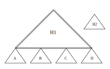
Phase I: Merge
Let represent 's height. Since , we can find a subheap of with the same height as . In the left diagram, subheaps , , , and are such heaps.
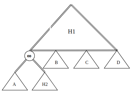
Since , we use Case I's strategy to merge into :
- Create a new heap and set the root 's priority to .
- Set and to be 's left and right child, respectively.
- Replace with this new heap.
We arrive at the right diagram.
Phase II: Adjust
To get rid of node, consider the following three nodes:
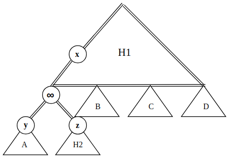
- Node : root of subheap .
- Node : root of subheap .
- Node : 's parent, which originally was 's parent.
We have the following observations:
and are valid heaps by construction, hence both satisfy the heap property.
By heap ordering property of , was 's parent previously implies , so subheap (and its root ) will not violate the heap property.
The only problem is we don't know about the relationship between and .
- If , then we can bubble up and call
deleteMax(). - If however, the heap ordering property is broken. Moreover, if , then there might exist more elements in that has a larger value than , or more ancestors of is less than .
- If , then we can bubble up and call
To fix the problem (when ):
For all ancestors of , call
fix-down(a).- This guarantees all ancestors of will be bubbled into the correct place.
- In the worst case, there are such ancestors (), and each
fix-down(a)requires comparisons (again, ), so overall this step takes .
Call
deleteMax(): After thosefix-down's, will be at the root position. CallingdeleteMax()effectively removes .
Overall, the runtime is dominated by those fix-down's and hence has runtime .
Case III. is full but is not.
This takes time. We omit this case.
Case IV. Both are not full.
We split into heaps that are full.
xxxxxxxxxx91A2/ \3B K4/ \ / \5C D k K6/ \ / \ / \ / \7C C E F K K K K8/ \ / \ /9C C C C G- In the above diagram, elements labeled with same letter are grouped into one full heap, e.g., the entire right subheap (labeled
k) is a full heap, and the nodeFitself is a heap (because we have nothing to group it with). - Since the heap is not full, there will always be a path from root to leaf, where each node on the path is a one-node heap. In the diagram above, this path is represented by
A -> B -> D -> E -> F. - Since the path has at least one-node heaps, overall we get full heaps.
- In the above diagram, elements labeled with same letter are grouped into one full heap, e.g., the entire right subheap (labeled
For each full subheap, merge them into using Case III. Since each merge takes and we have full heaps, we end up with time.
Conclusion Overall, the runtime is dominated by Case IV: time.
Expected Merge
Pseudocode
xxxxxxxxxx141heapMerge(r1, r2)2r1, r2: roots of two heaps, possibly NIL3return: root of merged heap451. if r1 is NIL return r262. if r2 is NIL return r173. if key(r2) > key(r1)84. randomly pick one child c of r195. replace subheap at c by heapMerge(c, r2)106. return r1117. else128. randomly pick one child d of r2139. replace subheap at d by heapMerge(r1, d)1410. return r2
- Assume heaps are stored as binary trees but with heap ordering property.
- We merge the heap with smaller root into the other one.
- We randomly choose the child at which to merge, then enter recursion.
Graphical Illustration
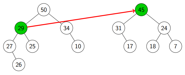
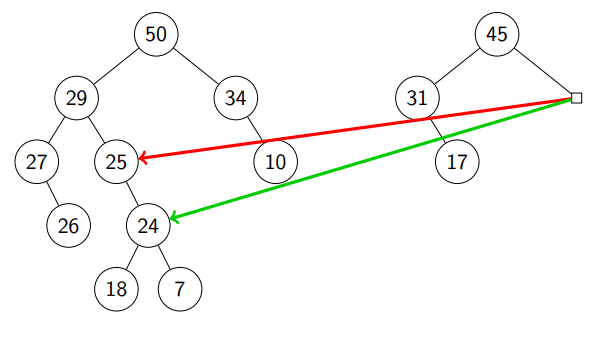
Suppose we want to merge the following two heaps.
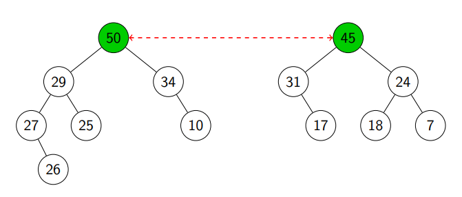
We see that root of left heap is greater than root of right heap (see line 7).
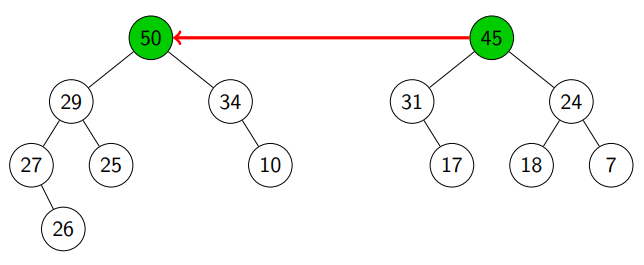
We randomly pick a child of and ended up with (see line 8).
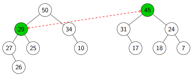
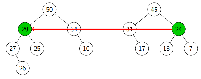
We see (see line 3).
We randomly pick a child of and ended up with (see line 4).
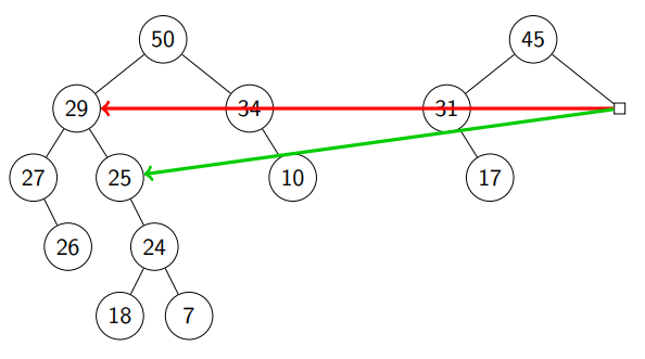
We keep doing this:
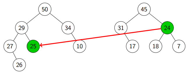
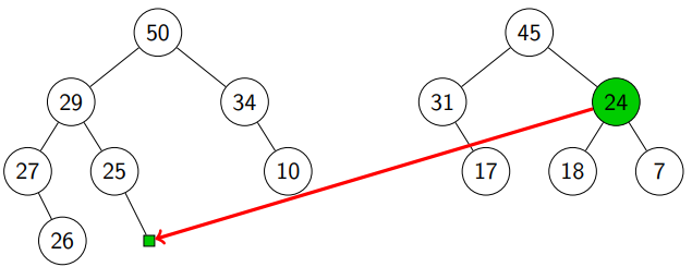
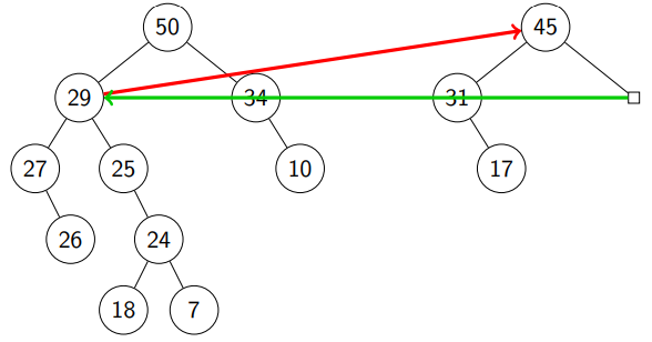
Finally, we see that r1 is NIL and move (subheap with root ).
Return from call stack:
Return from call stack & compare with : we move the subheap with root .
Return from call stack & compare with : we move the subheap with root .
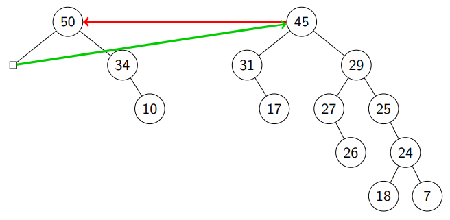
We are done!
Expected Runtime Analysis
Recall the expected runtime of a randomized algorithm can be expressed as:
We want to design the randomization such that all instances of size have equally good performance because the expected runtime depends on the of every instance.
Before we analyze the expected runtime of heap merge, let us first consider a simpler problem:
Problem Given a binary tree, you do a random walk downtime until you reach NIL. What is the runtime for this? We make no assumption on the tree, i.e., it may be very unbalanced.
Lemma The expected runtime (i.e., on a tree of nodes) is .
Proof. Assume that the time to go from a node to a randomly chosen child is at most . We claim that . We prove by induction.
Base: .
- LHS: because we are one step away from
NIL. - RHS: .
- LHS: because we are one step away from
Step: .
Let , represent the number of nodes in the left and right subtrees, respectively. Then .
The total runtime can be expressed s:
- : time for choosing child and walking down
- : probability of choosing the left subtree times the runtime when left subtree is chosen.
- : probability of choosing the right subtree times the runtime when right subtree is chosen.
Recall concave functions has the property that
Thus,
Back to the heap merge analysis, we can view it as going down in both heaps randomly until one hits a NIL child. Then
Binomial Heap
Recall that merge is easy for list ( for concatenation). To achieve our goal of worst-case merging, we can store a list of trees that satisfy the heap-property.
Binomial Tree

A binomial tree is defined recursively as follows:
- A binomial tree of order is a single node.
- A binomial tree of order has a root node whose children are roots of binomial trees of order (in this order).
Because of its unique structure, a binomial tree of order can be constructed from two trees of order trivially by attaching one of them as the left-most child of the root of the other tree. This feature is central to the merge operation of a binomial heap, which is its major advantage over the conventional heaps.
Remark. The name comes from the shape: a binomial tree of order has nodes at depth .
Claim. A binomial tree of order has nodes with height .
Proof. We prove by induction. The base case is trivial. Suppose this is true for . Then binomial tree contains two copies of , so has nodes. Because the max depth of a node in is one greater than the max depth in , by the inductive hypothesis, the maximum depth is .
Binomial Heap
A binomial heap is implemented as a set (or list, as presented in our class) of binomial trees that satisfy the binomial heap properties:
- Each binomial tree in a heap obeys the heap ordering property.
- There can only be either one or zero binomial trees for each order, include zero order.
The first property ensures that the root of each binomial tree contains the maximum in the tree, which applies to the entire heap.
The second property implies that a binomial heap with nodes consists of at most binomial trees. In fact, the number of orders of these trees are uniquely determined by the number of nodes : each binomial tree corresponds to the bits in the binary representation of number . For example, if a heap contains nodes, then this binomial heap with nodes will consist of three binomial trees of order , and .
Binomial Heap Operations
Let be the list of trees and be the degree at the root of tree (take the max).
Merge: as we are basically concatenating lists.
Insert: for the same reason. In fact, insertion can be seen as merging as well.
DeleteMax: ).
Locate the max: search among all roots, of them so for searching.
Remove the max and merge the subtrees into the heap: suppose the tree has children, then we need to perform insertions. Hence time for merging.
Cleanup: we want to merge trees together so after this step, no two trees have the same degrees in the list.
xxxxxxxxxx201binomialHeapCleanup(R, n)2R: stack of trees (of a binomial heap of size n)341. C <- array of length (log n + 1), initialized NIL52. while R is non-empty:63. T <- R.pop() // extract a tree to work with74. d_T <- degree of root of T // check how many children root of T has85. if C[d_T] is NIL // if we haven't found another tree of the same degree96. C[d_T] <- T // we put a pointer to T in the C[d_T]107. else // not NIL means we have saw another tree of the same degree118. T' <- C[d_T]; C[d_T] <- NIL // extract the previous result129. if key(root(T)) > key(root(T'))1310. make root(T') a child of root(T)1411. R.push(T)1512. else1613. make root(T) a child of root(T')1714. R.push(T')1815. for i<-0 to log n: // Finally, we merge the binomial trees together1916. if C[i] != NIL2017. R.push(C[i])
Amortized Analysis (via Potential Function)
Lemma. If all trees were built with these operations, .
Proof. . This also implies .
Define , where is the number of trees at time stamp and is a constant bigger than all constants in all other terms. Recall the amortized runtime of step is defined to be .
To show merge(R1, R2) has amortized time :
- Actual runtime: .
- Potential difference: , or the difference between number of trees at vs . Before the merge there are trees. Since we are not modifying anything (only moving them), there are still the same number of trees.
- Putting them together: .
Time to analyze deleteMax():
Actual time: .
Potential difference: , number of trees after minus number of trees before.
Putting them together:
where the finds the max degree of all trees that could be in a binomial heap with items.
Improvement on Worst-Case Performance
So far we have achieved amortized runtime for deleteMax(). If we are willing to trade runtime for merge/insert for deleteMax(), we can achieve worst-case for all three operations.
By calling clean-up after every operation (insert/merge), we can keep . Recall clean-up takes . Enforcing this would make insert/merge/deleteMax all achieve worst-case runtime.
Magic Trick
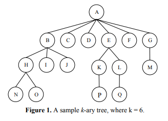
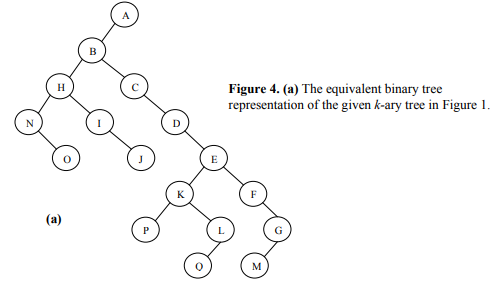
We can use a binary tree to store a tree with an arbitrary degree!
The new binary tree has the same nodes as . For node in , its left child in is the left-most child in and right child in is its sibling in .